Applied Nonlinear Control, slotine

https://web.mit.edu/nsl/www/videos/lectures.html

https://web.mit.edu/nsl/www/videos/lectures.html

 

1강 Introduction

 

세계의 시스템은 대부분 nonlinear이다.

 

 

Lyapunov theroy 리아프노프 : 러시아 수학자

일반적인 시스템

$$ \dot{x} = f(x)   :   autonomous,  time-invariant  $$

$$ \dot{x} = f(x, t)  :  non \; autonomous, time-varying $$ 

평형점(equilibrium point) :

$$ f(x_{eq}) = 0  : may \; have \; several \; solution! $$

 

ex) 3.1 pendulum 

 

pendulum

댐핑토크 : 진자의 회전 운동을 감쇄시키는 힘, 회전속도에 비례해 반대방향으로 작용

$$ torque_{damping} = -b\dot{\theta } \\ mR^2\ddot{\theta } = -mgsin(\theta)R-b\dot{\theta } \\ mR^2\ddot{\theta} + mgsin(\theta)R+b\dot{\theta }=0  $$

이를  state equation으로

$$ x_1=\theta \\ x_2=\dot{\theta } \\ \dot{x}_1 = x_2 $$

$$ \dot{x}_2 = \frac{-b}{mR^2}x_2 - \frac{g}{R}sin(x_1) $$

평형점은

$$ f(x)=0 \Leftrightarrow \begin{cases}
x_2=0 & \text{  } ,\dot{\theta} =0 \\ sin(x_1)=0
 & \text{} ,\theta=0 \; or \;\pi  
\end{cases} $$ 해가 여러 개 이다!

 

수학 기호

$$ \forall : for\; any \\ \exists : there \; exists \; at \; least \; one $$

W.L.O.G - Without Loss Of Generality : 특정 조건을 주더라도 문제 상황에 큰 영향이 없을 때, 풀이읭 용이함을 위해 조건을 맞추겠다는 의미

 

stability in the sense of lyapunov

리아프노프 안정성

ball centered at x=0, radius R

{$ {x, \left\| x \right\| < R} $}

$$ \forall R>0, \exists r>0 \\ if\;x(t=0) < r \\ then\;x(t) < R\;when\;\forall t > 0 $$

 

local asymptotic stability : 위의 조건 더하기

$$ \exists\;r_0 > 0\;such\;that \\ if\;x(t=0)<r_0 \\ then\;x(t)\to 0\;as\;t\rightharpoonup \infty  $$

asymptotic stability 에서 명백히 stability condition이 유지되었다.

 

global asymptotic stability : r_0가 무한대일때

 

exponential stability

starting in some ball of radius r_0

$$ \exists\alpha >0, \exists \lambda >0 $$ 알파는 큰 수, 람다는 시간관련

$$ such\;that\;\forall t\geq 0,\;\left\| x(t)\right\| \leq  \alpha \left\| x(t=0)\right\|e^{-\lambda t}$$

global : r_0가 무한대일때

$ Remark\; ; \; if\;\alpha =e^{\lambda \tau_0}\\then\;\alpha e^{-\lambda t}=e^{-\lambda (t-\tau_0)} $  tau_0는 extra delay

 

 

테일러 전개 : 다항식이 아닌 함수를 다항식으로 만드는 방법
* 함수가 0이 되지 않고 무한번 미분 가능한 함수만 가능

테일러 급수 : 테일러 전개로 얻은 다항식
$$ f(x)=\sum_{k=0}^{\infty}\frac{f^k(a)}{k!}(x-a)^k $$

매클로린 급수 : x=0에서 근사하는 테일러 전개의 특별한 경우
$$ f(x)=\sum_{k=0}^{\infty}\frac{f^k(0)}{k!}(x)^k $$

예) $$ f(x)=e^x $$ 이를 무한개의 식을 가진 다항식으로 표현할 수 있다고 가정
$ e^x = a_0 + a_1x + a_2x^2 + a_3x^3 +  \cdots\;\;x=0\;일\;때\;a_0=1 $
위 식을 미분하면
$ e^x=a_1+2a_2x+3a_3x^2+  \cdots\;\;x=0\;일\;때\;a_1=1 =\frac{1}{1}$
위 식을 미분하면
$ e^x=(2\cdot1)a_2+(3\cdot2)a_3x+  \cdots\;\;x=0\;일\;때\;a_2=\frac{1}{2!} $
$\Rightarrow e^x=1+x+\frac{x^2}{2!}+\frac{x^3}{3!}+\cdots $

 

2강

Linearization and Global stability

다음 시스템에서

$$  \dot{x}=f(x),\;f(0)=0 \\ \dot{x}=f(0) +\frac{\partial f}{\partial x}(x-0) + higher\;order\;term $$

이 때 f의 x에 대한 쟈코비안 : 밑의 A 행렬과 같음

$ \frac{\partial f}{\partial x}=\begin{pmatrix}
\frac{\partial f_1}{\partial x_1} & \cdots  & \frac{\partial f_1}{\partial x_n} \\
 \vdots &\ddots   & \vdots  \\
\frac{\partial f_n}{\partial x_1} & \cdots  & \frac{\partial f_n}{\partial x_n} \\
\end{pmatrix} $ 

첫 번째 행 : f_1의 gradient $ \nabla f_1 $

* gradient(기울기) : 함수의 각 성분의 편미분으로 구성된 벡터

linear approximation : $$  \dot{x}\approx Ax $$

 

다음과 같은 시스템에서

$$ \dot{x}=f(x, u) =f(0) +\frac{\partial f}{\partial x}(x-0) + \frac{\partial f}{\partial u}(u-0)  + higher\;order\;term $$

linear approximation : $$  \dot{x}\approx Ax + Bu $$

$$ if\;u(x)=k(x)=0+\frac{\partial k}{\partial x}(x-0) + higher\;order\;term \\u=kx$$

 

$$ \dot{x}=(A+Bk)x +h.o.t $$

 

ex) 3.4

$$ \dot{x_1}=x_2^2 + x_1cos(x_2) \\ \dot{x_2} = x_2 + (x_1 + 1)x_1 + x_1sin(x_2) $$

x=0이 평형점이다.

$$ \dot{x_1}\approx 0 + x_1\cdot1 = x_1 \\ \dot{x_2}= x_2 + 0+x_1 + x_1 x_2 \approx x_1 + x_2 $$

또한

$$  A = \begin{pmatrix}
\frac{\partial x_1}{\partial x_1} & \frac{\partial x_1}{\partial x_2} \\
\frac{\partial }{\partial x_1}(x_1 + x_2) & \frac{\partial }{\partial x_2}(x_1 + x_2) \\
\end{pmatrix} =  \begin{pmatrix}
1 & 0 \\
1 & 1 \\
\end{pmatrix}$$

 

 

lyapunov's linearization method

$$ \dot{x}=f(x)=Ax = h.o.t, \; f(0)=0 $$

만약 A가 restrictly stable하다면, 모든 고윳값은 LHP에 있다. 이러면 이 평형점은 점근적 안정

만약 A가 restrictly unstable 하다면, 적어도 A의 고윳값 중 하나는 RHP 에 있다. 이러면 X=0은 안정하지 않다.

만약 A가 marginally stable 하다면, 모든 고윳값은 LHP에 있지만 아마도 허수축에도 있을 수 도 있다.

 

 

lyapunov's direct method

 

nonlinear spring과 nonlinear damper 시스템

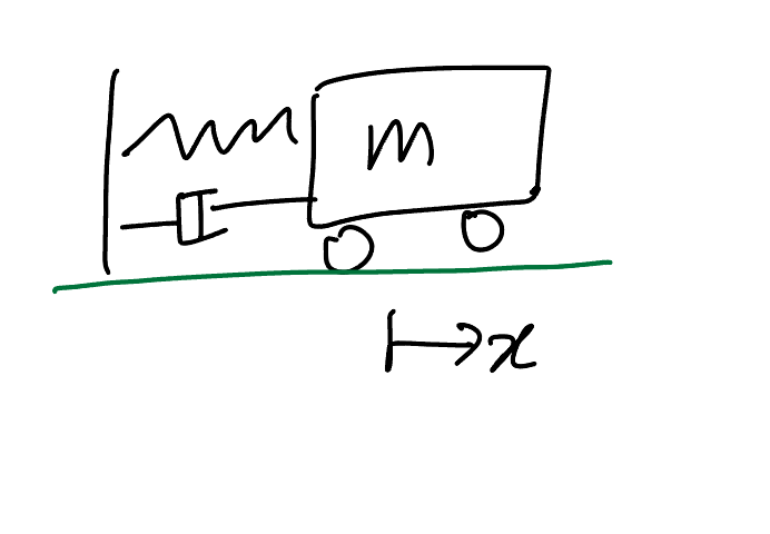
$$  m\ddot{x} + b\left| \dot{x}\right| \dot{x} + k_0x + k_1x^3 = 0 $$

이 때 평형은 x=0 과 x_dot = 0

총 에너지 = 키네틱 에너지 + 포텐셜 에너지

$$ V(x) =  \frac{1}{2}m\dot{x}^2 + \int_{0}^{x}(k_0y + k_1y)dy = \frac{1}{2}m\dot{x}^2 + \frac{k_0x^2}{2} + \frac{k_1x^4}{4} $$

V(x)는 스칼라이며 0보다 크거나 같고, V(x) 가 0인 것과 x=x_dot=0 은 동차이다.

 

$$ \frac{\mathrm{d} }{\mathrm{d} t}V(x) = m\dot{x}\ddot{x} + (k_0x + k_1x^3)\dot{x} = \dot{x}(-b\left| \dot{x}\right|\dot{x}-k_0x-k_1x^3) + (k_0x+k_1x^3)\dot{x} = \dot{x}(-b\left| \dot{x}\right|\dot{x})=-b\left| \dot{x}\right|^3\leq 0 $$

이 값은 nonlinear damper 에 의해 power가 dissipated(소멸)된 것이다.

 

 

3장

lyapunov's direct method

autonomous system 즉, time-invariant인 $$ \dot{x}=f(x) $$ 이 있고, 부드러운 스칼라 함수 V(x)에 대해

이다.

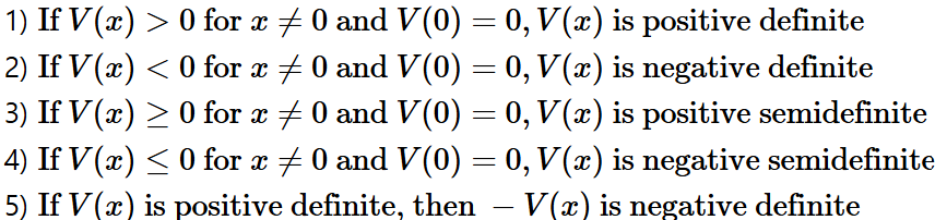
이 때  $$V(x)\;가\;positive\;definite\;이고\;\dot{V(x)}\;가\;negative\;semi\;definite\;라면 \\ 시스템은\;x=0\;에서\;stable\;하다.$$

$$ 만약\;\dot{V(x)}가\;negative\;definite\;라면\;시스템은\;x=0\;에서\;점근적으로\;stable\;하다$$

 

$$ 만약 \; r_0=\infty \; 라면 \; globally \; stable \; 하다.$$

 

ex)3.9

$$ \dot{x}+c(x)=0 \\ c(x) \; is \; continous, \; x \cdot c(x)>0 \;for \; x \neq 0 $$

$$ suppose \; V(x)=x^2, \; V \; is \; positive \; definite $$

$$ \dot{V(x)}=2x\dot{x}=-2x \cdot c(x)<0 \; for \; x \neq 0, \; \dot{V} \; is \; negative \; definite $$

$$ \left\| x\right\|\to \infty, \; V \to \infty \; : \; radial \; unboundness \; condition $$

$$ 평형점 \; : \; x=0, \; globally \; asymptotically \; stable $$

 

$$ \dot{x}=-x^3, \; c(x)=x^3, \; G.A.S \\ Linearization \; : \; \dot{x}=0, \; marginally \; stable $$

$$ \dot{x}+x=sin^2(x) \; c(x)=x-sin^2(x), \; G.A.S \\ because \; sin^2(x) \leq  \left| sin(x)\right| <  \left| x \right| \; for \; x \neq 0 $$