Vector Spaces

 

교재 : Linear System Theory and Design $4_{th}$ Ed. by Chen, Oxford, 2013

 

Vector space

스칼라 필드 $\textit{K} (실수 or 복소수)$에 대한 Vector space $\textit{V}$

Definition : $\textit{V}$ 는 공집합이 아니며

1. Vector Addition : for any $\textit{u, v} \in V$, a sum  $\textit{u+v} \in V$

2. Scalar Multiplication : any $\textit{u} \in V$,  $\textit{k} \in K$, a product  $\textit{ku} \in V$

 

 $\textit{u, v, w} \in V$ : vector space에 있는 element를 vector 라고 부른다.

 

8가지 공리를 만족

1. $(u+v) + w = u + (v+w)$ : 결합 법칙, associativity

2. for any  $\textit{u} \in V$, zero vector, 영벡터

$$u+0 = 0+u = u$$

3. for each $\textit{u} \in V$, $negative$ of $u$, $-u$

$$u+(-u)=(-u)+u=0$$

4. $u+v=v+u$

5. for any scalar $\textit{k} \in K$, $k(u+v)=ku+kv$, 분배 법칙

6. for any scalars $\textit{a, b} \in K$, $(a+b)u=au+bu$

7. for any scalars $\textit{a, b} \in K$, $(ab)u=a(bu)$

8. for the unit scalar $\textit{1} \in K$, $1u=u$

 

Vector space의 예시

1. 유클리드 공간 Euclidean space

definition : 유클리드 공간은 $\mathbb{R}^n$ 으로 정의되는 특정한 vector space로, 다음과 같은 추가적인 구조가 정의된 공간

- 내적 : 두 벡터간 내적 $u\cdot v$가 정의됨.

            이를 통해 벡터의 크기$($길이$)$와 각도를 계산할 수 있음

- 거리와 크기 : 벡터의 크기 norm은 $\left\| v\right\| = \sqrt{v\cdot v}$

                        두 벡터 사이의 거리, 유클리디안 거리 $d(u,v)=\left\| u-v\right\|$

- 예시 : $\mathbb{R}^2$ : 2차원 평면 공간, x-y좌표

            $\mathbb{R}^3$ : 3차원 평면 공간. x-y-z 좌표   

 

space $K^n$, 즉 K가 실수라면 $R^n$은 유클리디안 공간이고 이는 vector space 이다.

 

vector addition과 scalar multiplication을 각각의 space에 대해 정의해야 한다.

vector addition : $(a_1,a_2, \cdots , a_n)+(b_1,b_2, \cdots. b_n) = (a_1+b_1. a_2+b_2, \cdots, a_n+b_n)$

scalar multiplication : $k(a_1,a_2, \cdots , a_n) = (ka_1, ka_2, \cdots, ka_n)$

 

2. Polynomial space $P_n(t)$

스칼라 필드 K에 대한 모든 다항식 $p(t)$의 집합 $P_n(t)$ 는 차수가 n이하인 모든 다항식

$P(t) = a_0 + a_1t + a_2t^2+ \cdots + a_st^s$

vector addition, scalar multiplication은 다항식에 대해 성립

 

3. Matrix space $M_{m,n}$

스칼라 필드 K에 대한 모든 $m x n$ matrix들의 집합

vector addition, scalar multiplication 성립

 

4. Function space $F(X)$

다항식을 비롯한 모든 함수가 포함됨

vector addition, scalar multiplication 성립

 

Linear Dependence and Independence 선형 의존, 선형 독립

definition : 만약 scalar $a_1, a_2, \cdots , a_m$ 이 K에서 존재하고, 

$a_1v_1 + a_2v_2 + \cdots + a_mv_m = 0$ only when $a_1 = a_2 = \cdots = 0$이라면

 vectors $v_1, v_2. \cdots ,v_m$ in V  는 linearly independenet 하다. 

그게 아니면, linearly dependent 하다. 

 

Linear Combination 선형 조합

V는 스칼라장 K에 대한 vector space 이고, vector v in V is a linear combination of vectors $u_1, u_2, \cdots, u_m$ in V if there exist scalars $a_1, a_2, \cdots, a_m$ in K such  that

$$v = a_1u_1 + a_2u_2 + \cdots + a_mu_m$$

 

Spanning Sets 생성 집합

모든 가능한 linear combination

 

given $u1, u2, span\left\{u_1,u_2 \right\} = \left\{ au_1+bu_2 | a,b \in K \right\}$

 

Subspaces 부분 공간

subspace = subset of vector spaces, 또한 그것 자체도 vector space

모든 subspace는 원점을 지나야 한다!

예) vector space $V=R^2$

subset A : scalar multiplication 이 안됨, 영벡터가 포함 안됨

A는 V의 subspace가 아니고, vector space가 아니다.

 

subset C : 직선

vector addition, scalar multiplication 이 가능해 vector space이고, $V=R^2$의 subspace 이다.

 

V의 subspace들의 합집합은 V의 subspace가 아니고, 교집합은 subspace가 맞다.

 

 

행렬 A에 대한 row space : 행렬 A의 row의 linear combination으로 만들 수 있는 모든 집합. span{rows}

Let $A = \begin{bmatrix} 2 & -1 & 0 \\ 2 & 1 & 0 \\ 0 & 1 & 1 \\ \end{bmatrix}$

우선 A를 echelon form으로 변환해야 한다.

L2 = L2 - L1

A = $\begin{bmatrix} 2 & -1 & 0 \\ 0 & 2 & 0 \\ 0 & 1 & 1 \\ \end{bmatrix}$

L3 = 2*L3-L2

 A = $\begin{bmatrix} 2 & -1 & 0 \\ 0 & 2 & 0 \\ 0 & 0 & 2 \\ \end{bmatrix}$

 

row space of A = span{ $\begin{pmatrix} 2 \\ -1 \\ 0 \end{pmatrix}, \begin{pmatrix} 0 \\ 2 \\ 0 \end{pmatrix},  \begin{pmatrix} 0 \\ 0 \\ 2 \end{pmatrix}$ }

만약 행렬 A의 row vector 들이 서로 linearly independent이면 row space의 basis가 된다.

행렬의 Row Space를 구성할 때, 각 행$row vector$이 꼭 선형 독립일 필요는 없습니다. 하지만, Row Space의 **기저$basis$**를 구성하는 벡터들은 반드시 선형 독립이어야 합니다.

 

행렬 A에 대한 column space

$A^T = \begin{bmatrix} 2 & 2 & 0 \\ -1 & 1 & 1 \\ 0 & 0 & 1 \\ \end{bmatrix}$

L2 = L1 + 2*L2

$A^T = \begin{bmatrix} 2 & 2 & 0 \\ 0 & 4 & 2 \\ 0 & 0 & 1 \\ \end{bmatrix}$

 

column space of A = span{ $\begin{pmatrix} 2 \\ 2 \\ 0 \end{pmatrix}, \begin{pmatrix} 0 \\ 4 \\ 2 \end{pmatrix},  \begin{pmatrix} 0 \\ 0 \\ 1 \end{pmatrix}$ }

 

A의 row vector를 span한 row space는, A를 전치한 $A^T$의 column vector를 span한 column space와 같다.

 

Ax=b 는 모든 b 에 대해 해를 가지고 있을까?

우측의 형태는 A의 column의 선형 결합과 형태가 같다.

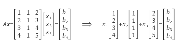
예를 들어 b = [0 0 0 0$]^T$ 일 때 x = [0 0 0$]^T$ 가 된다.

또한 b=[1 2 3 4$]^T$ 일 때 x=[1 0 0$]^T$이 된다. 이때 b는 A의 첫 번째 열과 같다.

 

우리는 선형 방정식 Ax=b에 대해 b벡터가 A의 column space에 존재할 때만 해를 구할 수 있다.
즉, b벡터가 A의 column의 linear combination으로 표현이 가능할 때 Ax=b에 대한 해를 구할 수 있다.

 

 

Gauss Elimination 가우스 소거법

gauss elimination, 즉 row reduction이란, 연립일차방정식을 풀이하는 알고리즘이다. 풀이 과정에서, 일부 미지수가 차츰 소거되어 결국 남은 미지수에 대한 linear combination으로 표현되면서 풀이가 완성된다.

 

row operations

1. 두 행을 바꾼다

2, 한 행에 0이 아닌 스칼라를 곱한다

3. 한 행에 스칼라를 곱하고 다른 행으로 더한다.

 

echelon : 계급, 계층, 지위

in echelon : 사다리꼴을 이루어

row echelon form

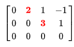
row echelon form 행사다리꼴 행렬 은 gauss elimination의 결과로 얻어지는 행렬이다.

조건 1. 0으로만 이루어진 행이 존재할 경우에 그 행은 행렬의 마지막 행이다.

        2. 모든 0이 아닌 행의 pivot , 즉 leading coefficient 선행계수는 항상 그 위 행의 선행계수의 오른쪽에 있다.

* 만약 이때 모든 pivot이 1이면 reduced row echelon form 이다.

 

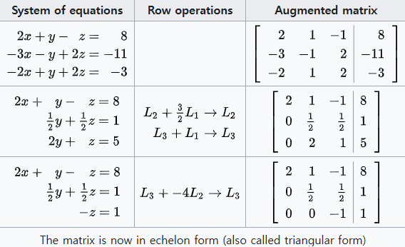
row reduction 절차 : 1행 밑에서 x를 제거한다, 그 후 2행 밑에서 y를 제거한다.

시스템을 triangular form으로 만든 이후 back substitution을 통해 각각의 미지수를 푼다.

 

Basis and Dimension

basis 기저

definition : A set $S = {u_1, u_2, \cdots, u_n}$ of vectors is a basis  of V if it has the following two properties : 

1. S is linearly independent, 최소한의 개수

2. S spans V

 

dimension 차원 : 벡터 공간에서 차원은 선형 독립 벡터들로 이루어진 basis의 개수 로 정의된다.

즉, 차원은 벡터 공간을 생성 span 하는 데 필요한 최소한의 벡터 수 이다.

 

단일 벡터 자체에는 차원이 정의되지 않는다.

하지만 단일 벡터 $v \neq 0$로 생성된 벡터 공간의 차원은 1이다.

단일 벡터가 영벡터라면, 생성된 벡터 공간의 차원은 0이다.

 

 

vector space $M_{2,3}$ 의 경우 basis :

$\begin{bmatrix} 1& 0 & 0 \\0 & 0 & 0 \\ \end{bmatrix}, \begin{bmatrix} 0 & 1 & 0 \\0 & 0 & 0 \\ \end{bmatrix}, \begin{bmatrix} 0 & 0 & 1 \\0 & 0 & 0 \\ \end{bmatrix}, \begin{bmatrix} 0 & 0 & 0 \\1 & 0 & 0 \\ \end{bmatrix}, \begin{bmatrix} 0 & 0 & 0 \\0 & 1 & 0 \\ \end{bmatrix}, \begin{bmatrix} 0 & 0 & 0 \\0 & 0 & 1 \\ \end{bmatrix}$ 

 

차원 $dim M_{2,3} = 2 \times 3 = 6$

 

vector space $P_n(t)$ of all polynomials of degree $\leq n$ 의 경우 

n+1차 polynomial의 set S = {$1, t, t^2, t^3 , \cdots, t^n$} 가 basis

 

차원 $dim P_n(t) =  n+1$

 

Rank of matrics

definition : The $rank$ of a matrix A, written rank$A$, is equal to the maximum number of linearly independent rows/columns of A

$$rank(A) = rank(A^T)$$

 

$A = \begin{bmatrix} 1&2 \\ 2&3 \\ 3&0  \end{bmatrix}$

 

$-6(\frac{3}{2}L_1 - L_2) = L_3$, L1과 L2는 linearly independent

$rank(A) = 2$

 

$B = \begin{bmatrix} 1&10 \\ 2&20 \\ 3&30  \end{bmatrix}$

$rank(B) = 1$, 최소 rank는 1이다.

 

matrix를 row reduction form으로 만들면 pivot column의 개수가 그 matrix의 rank 이다.

$A = \begin{bmatrix} 1&2 \\ 2&3 \\ 3&0  \end{bmatrix}$

L2 = L2-2*L1 하면

$RREF(A) = \begin{bmatrix} 1&2 \\ 0&-1 \\ 3&0  \end{bmatrix}$

L3=L3-3*L1하면

$RREF(A) = \begin{bmatrix} 1&2 \\ 0&-1 \\ 0&-6  \end{bmatrix}$

L3=L3-6*L2하면

$RREF(A) = >\begin{bmatrix} 1&2 \\ 0&-1 \\ 0&0  \end{bmatrix}$

RREP$A$에 2개의 pivot column이 있으므로 A의 rank는 2이다.

 

A "pivot column" in a matrix is 
a column that contains a "pivot element", which is the leading non-zero entry in a row when the matrix is in row echelon form

 

Sums and direct sums

sum

U+W = {v : v = u+w, where $u \in U$ and $w \in W$ }

U와 W는 V의 subspace이면, U+W 도 V의 subspace이다.

$dim(U+W) = dim U + dim W - dim(U \cap W)$

 

$U={1, 2}, W={3, 4}$ 이면 $U +W = {1+2, 1+3, 2+3, 2+4}, U \cup W = {1, 2, 3, 4}$

 

direct sum

vector space V는 V의 subspace U와 W의 direct sum 이다. $V = U \oplus  W$ 오직 다음 두 조건을 만족할 때 : 

1. $V=U+W$

2. $U \cap W = {0}$

영벡터는 모든 vector space의 필수적 구성 요소로, 공간의 독립성을 깨지 않는다.

Coordinates 좌표

V가 basis $S={u_1,u_2,\cdots,u_n}$인 n-dimensional vector space라 하자.

그러면 any vector $v \in V$는 basis vector S의 linear combination으로써 유일하게 표현될 수 있다.

$$v = a_1u_1 + a_2u_2 + \cdots + a_nu_n$$

이런 n개의 scalar $a_1,a_2,\cdots,a_n$을 vector v의 basis S에 상대적인 coordinates 라고 한다. 주로 열벡터로 표현된다.